
🔥Machine Learning Course🔥
Computer Vision – From OpenCV to SOTA
Chào mọi người. Mình là Minh. Đây là bài viết bài viết đầu tiên của mình trong chuỗi bài về Thị giác máy tính. Mình dành thời gian viết chuỗi bài này để giới thiệu tới mọi người những kiến thức nhỏ mà mình học được. Hy vọng nó sẽ giúp ích với mọi người.
Part I: From OpenCV to Convolutional Neural Network for Computer Vision
Table of Content
Applications of Computer Vision
Các ứng dụng của thị giác máy tính bao gồm tự động hóa trong các phương tiện tự lái đến phát triển phần mềm nhận dạng chính xác để kiểm tra sản phẩm trong dây chuyền sản xuất sản xuất đến điều khiển robot, tổ chức thông tin, chẳng hạn như lập chỉ mục cơ sở dữ liệu hình ảnh.
Thị giác máy tính, cũng như các khái niệm về AI và học máy, là chìa khóa để hiện thực hóa quá trình tự động hóa hoàn chỉnh, hoặc Cấp độ 5 trong các phương tiện tự lái. Tại đây phần mềm CV phân tích dữ liệu từ các camera đặt xung quanh xe. Điều này cho phép chiếc xe xác định các phương tiện khác và người đi bộ cũng như đọc các biển báo đường bộ. Thị giác máy tính cũng là chìa khóa để phát triển phần mềm nhận dạng khuôn mặt chính xác. Điều này thường xuyên được các cơ quan thực thi pháp luật thực hiện cũng như giúp xác thực quyền sở hữu thiết bị của người tiêu dùng.
Công nghệ thực tế tăng cường và hỗn hợp đang ngày càng được triển khai trên điện thoại thông minh và máy tính bảng. Hay như smart glass cũng đang trở nên phổ biến rộng rãi hơn. Tất cả những điều này đòi hỏi thị giác của máy tính để giúp xác định vị trí, phát hiện các đối tượng và thiết lập độ sâu hoặc kích thước của thế giới ảo. Trong khuôn khổ bài viết này, dữ liệu được mình sử dụng ngẫu nhiên, do đó nếu bạn muốn thử, hãy sử dụng dữ liệu của bạn. Hay thử tinh chỉ code của mình với dữ liệu của bạn để xem có gì bất ngờ xảy ra nhé 😊
Bài viết này yêu cầu kỹ năng lập trình với ngôn ngữ python ở mức độ cơ bản/ trung bình. Let’s get it started.
Understanding Images.
OpenCV (CV2) là một thư viện cực kỳ nổi tiếng cho các ứng dụng thị giác máy tính. Bạn có thể xem mã nguồn và hướng dẫn tại đây nè
NumPy là một thư viện phục vụ cho khoa học máy tính của Python, hỗ trợ cho việc tính toán các mảng nhiều chiều, có kích thước lớn với các hàm đã được tối ưu áp dụng lên các mảng nhiều chiều đó. Numpy đặc biệt hữu ích khi thực hiện các hàm liên quan tới Đại Số Tuyến Tính.
import numpy as np
import matplotlib.image as mpimg
import matplotlib.pyplot as plt
import cv2
%matplotlib inline
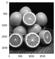
# Read in the image
image = mpimg.imread('images/oranges.jpg')
# Print out the image dimensions
print('Image dimensions:', image.shape)
plt.imshow(image)

# Change from color to grayscale
gray_image = cv2.cvtColor(image, cv2.COLOR_RGB2GRAY)

plt.imshow(gray_image, cmap='gray')
# Specific grayscale pixel values
# Pixel value at x = 400 and y = 300
x = 200
y = 100
print(gray_image[y,x])12
>>> 6
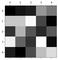
# 5x5 image using just grayscale, numerical values
tiny_image = np.array([[0, 20, 30, 150, 120],
[200, 200, 250, 70, 3],
[50, 180, 85, 40, 90],
[240, 100, 50, 255, 10],
[30, 0, 75, 190, 220]])
# To show the pixel grid, use matshow
plt.matshow(tiny_image, cmap='gray')
Images and Colors
In [7]:
# Read in the image
image = mpimg.imread('images/rainbow_flag.jpg')

plt.imshow(image)

RGB Channels
In [8]:
# Isolate RGB channels
r = image[:,:,0]
g = image[:,:,1]
b = image[:,:,2]

# The individual color channels
f, (ax1, ax2, ax3) = plt.subplots(1, 3, figsize=(20,10))
ax1.set_title('R channel')
ax1.imshow(r, cmap='gray')
ax2.set_title('G channel')
ax2.imshow(g, cmap='gray')
ax3.set_title('B channel')
ax3.imshow(b, cmap='gray')

Color Threshold
IIMG_PATH='introcv/'
image = cv2.imread(IMG_PATH+'images/pizza_bluescreen.jpg')
print('This image is:', type(image), ' with dimensions:', image.shape)

>>> This image is: <class 'numpy.ndarray'>  with dimensions: (514, 816, 3)

image_copy = np.copy(image)

# RGB (from BGR)
image_copy = cv2.cvtColor(image_copy, cv2.COLOR_BGR2RGB)

# Display the image copy
plt.imshow(image_copy)

# Color Threshold
lower_blue = np.array([0,0,200])
upper_blue = np.array([50,50,255])
Mask
# Define the masked area

mask = cv2.inRange(image_copy, lower_blue, upper_blue)

# Vizualize the mask

plt.imshow(mask, cmap='gray')

# Masking the image to let the pizza show through

masked_image = np.copy(image_copy)

masked_image[mask != 0] = [0, 0, 0]

plt.imshow(masked_image)

# Loading in a background image, and converting it to RGB

background_image = cv2.imread(IMG_PATH+'images/space_background.jpg')

background_image = cv2.cvtColor(background_image, cv2.COLOR_BGR2RGB)

# Cropping it to the right size (514x816)

crop_background = background_image[0:514, 0:816]

# Masking the cropped background so that the pizza area is blocked

crop_background[mask == 0] = [0, 0, 0]

# Displaying the background

plt.imshow(crop_background)

# Adding the two images together to create a complete image!
complete_image = masked_image + crop_background

# Displaying the result
plt.imshow(complete_image)

HSV
 image = cv2.imread(IMG_PATH+'images/water_balloons.jpg')

image_copy = np.copy(image)

image = cv2.cvtColor(image_copy, cv2.COLOR_BGR2RGB)

plt.imshow(image)

# Converting from RGB to HSV
hsv = cv2.cvtColor(image, cv2.COLOR_RGB2HSV)

# HSV channels
h = hsv[:,:,0]
s = hsv[:,:,1]
v = hsv[:,:,2]

f, (ax1, ax2, ax3) = plt.subplots(1, 3, figsize=(20,10))

ax1.set_title('Hue')
ax1.imshow(h, cmap='gray')

ax2.set_title('Saturation')
ax2.imshow(s, cmap='gray')

ax3.set_title('Value')
ax3.imshow(v, cmap='gray')

# Color selection criteria in HSV values for getting only Pink balloons
lower_hue = np.array([160,0,0])
upper_hue = np.array([180,255,255])

# Defining the masked area in HSV space
mask_hsv = cv2.inRange(hsv, lower_hue, upper_hue)

# masking the image
masked_image = np.copy(image)
masked_image[mask_hsv==0] = [0,0,0]

# Vizualizing the mask
plt.imshow(masked_image)

Classifying Images based on Features
In [21]:
# Helper function
import glob # hàm giúp load image từ directory

# This function loads in images and their labels and places them in a list
# The list contains all images and their associated labels
# For example, after data is loaded, im_list[0][:] will be the first image-label pair in the list

def load_dataset(image_dir):

    # Populate this empty image list
    im_list = []
    image_types = ["day", "night"]

    # Iterate through each color folder
    for im_type in image_types:

        # Iterate through each image file in each image_type folder
        # glob reads in any image with the extension "image_dir/im_type/*"
        for file in glob.glob(os.path.join(image_dir, im_type, "*")):

            # Read in the image
            im = mpimg.imread(file)

            # Check if the image exists/if it's been correctly read-in
            if not im is None:
          	# Append the image, and it's type (red, green, yellow) to the imgae list
                im_list.append((im, im_type))

    return im_list
## Standardizing the input images
# Resizing each image to the desired input size: 600x1100px (hxw).

## Standardizing the output
# With each loaded image, we also specify the expected output.
# For this, we use binary numerical values 0/1 = night/day.


# This function should take in an RGB image and return a new, standardized version
# 600 height x 1100 width image size (px x px)
def standardize_input(image):

    # Resize image and pre-process so that all "standard" images are the same size
    standard_im = cv2.resize(image, (1100, 600))

    return standard_im


# Examples:
# encode("day") should return: 1
# encode("night") should return: 0
def encode(label):

    numerical_val = 0
    if(label == 'day'):
        numerical_val = 1
    # else it is night and can stay 0

    return numerical_val

# using both functions above, standardize the input images and output labels
def standardize(image_list):

    # Empty image data array
    standard_list = []

    # Iterate through all the image-label pairs
    for item in image_list:
        image = item[0]
        label = item[1]

        # Standardize the image
        standardized_im = standardize_input(image)

        # Create a numerical label
        binary_label = encode(label)

        # Append the image, and it's one hot encoded label to the full, processed list of image data
        standard_list.append((standardized_im, binary_label))

    return standard_list
Day and Night Image Classifier
Bộ dữ liệu hình ảnh ngày/đêm bao gồm 200 hình ảnh màu RGB. Mỗi ví dụ có số lượng bằng nhau: 100 hình ảnh ngày và 100 hình ảnh ban đêm.</br>
Xây dựng một công cụ phân loại có thể gắn nhãn chính xác những hình ảnh này là ngày hay đêm và điều đó dựa vào việc tìm ra các đặc điểm phân biệt giữa hai loại hình ảnh!
Note: data is here: AMOS dataset
Training and Testing Data
Chia thành tập training và testing
• 60% là traning
• 40% là testing
image_dir_training = "introcv/day_night_images/training/"
image_dir_test = "introcv/day_night_images/test/"
# Load training data
IMAGE_LIST = load_dataset(image_dir_training)
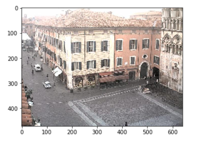
Visualizing an Image
image_index = 20
selected_image = IMAGE_LIST[image_index][0]
selected_label = IMAGE_LIST[image_index][1]
print(len(IMAGE_LIST))
print(selected_image.shape)
plt.imshow(selected_image)
Preprocessed images with labels
STANDARDIZED_LIST = standardize(IMAGE_LIST)
image_num = 0
selected_image = STANDARDIZED_LIST[image_num][0]
selected_label = STANDARDIZED_LIST[image_num][1]

# show ảnh
plt.imshow(selected_image)
print("Shape: "+str(selected_image.shape))
print("Label [1 = day, 0 = night]: " + str(selected_label))

Feature Extraction
# Chuyển sang không gian màu HSV
# Mô tả các kênh màu riêng lẻ

image_num = 0
test_im = STANDARDIZED_LIST[image_num][0]
test_label = STANDARDIZED_LIST[image_num][1]

hsv = cv2.cvtColor(test_im, cv2.COLOR_RGB2HSV)

print('Label: ' + str(test_label))

# HSV channels
h = hsv[:,:,0]
s = hsv[:,:,1]
v = hsv[:,:,2]

# Vẽ ảnh gốc và 3 kênh
f, (ax1, ax2, ax3, ax4) = plt.subplots(1, 4, figsize=(20,10))
ax1.set_title('Standardized image')
ax1.imshow(test_im)
ax2.set_title('H channel')
ax2.imshow(h, cmap='gray')
ax3.set_title('S channel')
ax3.imshow(s, cmap='gray')
ax4.set_title('V channel')
ax4.imshow(v, cmap='gray')

def avg_brightness(rgb_image):
    hsv = cv2.cvtColor(rgb_image, cv2.COLOR_RGB2HSV)

    # Cộng tất cả các giá trị pixel trong 3 kênh
    sum_brightness = np.sum(hsv[:,:,2])
    area = 600*1100.0  # pixels

    avg = sum_brightness/area

    return avg

# test giá trị sáng trung bình

image_num = 190
test_im = STANDARDIZED_LIST[image_num][0]

avg = avg_brightness(test_im)
print('Avg brightness: ' + str(avg))
plt.imshow(test_im)

Classifier
# This function should take in RGB image input
def estimate_label(rgb_image):

    # Extracting average brightness feature from an RGB image
    avg = avg_brightness(rgb_image)

    # Using the avg brightness feature to predict a label (0, 1)
    predicted_label = 0
    threshold = 98
    if(avg > threshold):
        # if the average brightness is above the threshold value, we classify it as "day"
        predicted_label = 1
    # else, the pred-cted_label can stay 0 (it is predicted to be "night")

    return predicted_label
Testing Classifier
import random

# Load test data
TEST_IMAGE_LIST = load_dataset(image_dir_test)

# Standardize the test data
STANDARDIZED_TEST_LIST = standardize(TEST_IMAGE_LIST)

# Shuffle the standardized test data
random.shuffle(STANDARDIZED_TEST_LIST)
Determining Accuracy
def get_misclassified_images(test_images):
    # Tracking misclassified images by placing them into a list
    misclassified_images_labels = []

    # Iterating through all the test images
    for image in test_images:

        im = image[0]
        true_label = image[1]

        predicted_label = estimate_label(im)

        # Comparing true and predicted labels
        if(predicted_label != true_label):
            # If these labels are not equal, the image has been misclassified
            misclassified_images_labels.append((im, predicted_label, true_label))

    return misclassified_images_labels

MISCLASSIFIED = get_misclassified_images(STANDARDIZED_TEST_LIST)

# Accuracy calculations
total = len(STANDARDIZED_TEST_LIST)
num_correct = total - len(MISCLASSIFIED)
accuracy = num_correct/total

print('Accuracy: ' + str(accuracy))
print("Number of misclassified images = " + str(len(MISCLASSIFIED)) +' out of '+ str(total))
Accuracy: 0.91875 Number of misclassified images = 13 out of 160
Image Filters
Fourier Transforms
Các thành phần tần số của hình ảnh có thể được hiển thị sau khi thực hiện Biến đổi Fourier (FT). FT xem xét các thành phần của hình ảnh (các cạnh có tần số cao và các vùng có màu mịn là tần số thấp) và vẽ biểu đồ tần số xuất hiện dưới dạng các điểm trong quang phổ.
Trên thực tế, FT coi các mẫu cường độ trong hình ảnh là sóng hình sin với một tần số cụ thể và bạn có thể xem hình ảnh trực quan thú vị về các thành phần sóng hình sin này ở đây.
Fourier Transform là một công cụ xử lý hình ảnh quan trọng được sử dụng để phân rã hình ảnh thành các thành phần sin và cosine của nó. Đầu ra của phép biến đổi đại diện cho hình ảnh trong miền Fourier hoặc miền tần số, trong khi hình ảnh đầu vào là miền không gian tương đương. Trong ảnh miền Fourier, mỗi điểm biểu diễn một tần số cụ thể có trong ảnh miền không gian.
Fourier Transform được sử dụng trong một loạt các ứng dụng, chẳng hạn như phân tích hình ảnh, lọc hình ảnh, tái tạo hình ảnh và nén hình ảnh.
Và một chút toán học ở đây:
Image Transforms - Fourier Transform
But what is the Fourier Transform? A visual introduction.
image_stripes = cv2.imread(IMG_PATH+'images/stripes.jpg')
image_stripes = cv2.cvtColor(image_stripes, cv2.COLOR_BGR2RGB)

image_solid = cv2.imread(IMG_PATH+'images/pink_solid.jpg')
image_solid = cv2.cvtColor(image_solid, cv2.COLOR_BGR2RGB)
Displaying
f, (ax1,ax2) = plt.subplots(1, 2, figsize=(10,5))

ax1.imshow(image_stripes)
ax2.imshow(image_solid)

# chuyển đổi sang thang độ xám để tập trung vào các mẫu cường độ trong hình ảnh
gray_stripes = cv2.cvtColor(image_stripes, cv2.COLOR_RGB2GRAY)
gray_solid = cv2.cvtColor(image_solid, cv2.COLOR_RGB2GRAY)

# chuẩn hóa các giá trị màu của hình ảnh trong phạm vi từ [0,255] đến [0,1]

norm_stripes = gray_stripes/255.0
norm_solid = gray_solid/255.0

# thực hiện biến đổi fourier nhanh
# và tạo hình ảnh biến đổi tần số được chia tỷ lệ

def ft_image(norm_image):
    '''This function takes in a normalized, grayscale image
       and returns a frequency spectrum transform of that image. '''
    f = np.fft.fft2(norm_image)
    fshift = np.fft.fftshift(f)
    frequency_tx = 20*np.log(np.abs(fshift))

    return frequency_tx

f_stripes = ft_image(norm_stripes)
f_solid = ft_image(norm_solid)

# displaying the images
# ảnh gốc ở bên trái biến đổi tần số của chúng

f, (ax1,ax2,ax3,ax4) = plt.subplots(1, 4, figsize=(20,10))

ax1.set_title('original image')
ax1.imshow(image_stripes)
ax2.set_title('frequency transform image')
ax2.imshow(f_stripes, cmap='gray')

ax3.set_title('original image')
ax3.imshow(image_solid)
ax4.set_title('frequency transform image')
ax4.imshow(f_solid, cmap='gray')
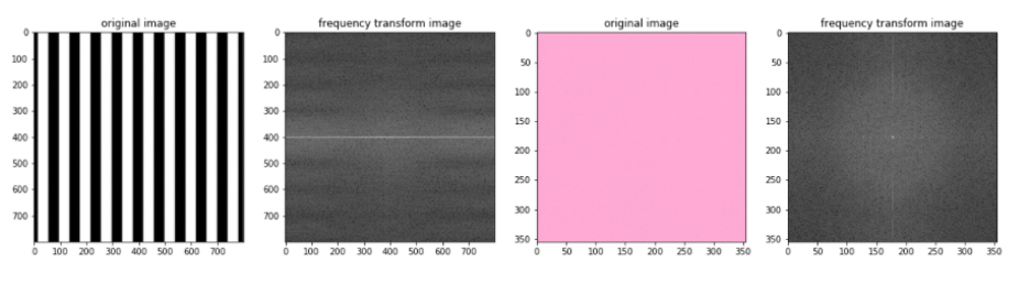
image = cv2.imread(IMG_PATH+'images/brain_MR.jpg')

image_copy = np.copy(image)

image_copy = cv2.cvtColor(image_copy, cv2.COLOR_BGR2RGB)

plt.imshow(image_copy)

Converting to grayscale for filtering
gray = cv2.cvtColor(image_copy, cv2.COLOR_RGB2GRAY)

# Creating a Gaussian blurred image
gray_blur = cv2.GaussianBlur(gray, (9, 9), 0)

f, (ax1, ax2) = plt.subplots(1, 2, figsize=(20,10))

ax1.set_title('original gray')
ax1.imshow(gray, cmap='gray')

ax2.set_title('blurred image')
ax2.imshow(gray_blur, cmap='gray')

High-pass filter
# 3x3 sobel filters for edge detection
sobel_x = np.array([[ -1, 0, 1],
                   [ -2, 0, 2],
                   [ -1, 0, 1]])


sobel_y = np.array([[ -1, -2, -1],
                   [ 0, 0, 0],
                   [ 1, 2, 1]])


# Filters the orginal and blurred grayscale images using filter2D
filtered = cv2.filter2D(gray, -1, sobel_x)

filtered_blurred = cv2.filter2D(gray_blur, -1, sobel_y)
f, (ax1, ax2) = plt.subplots(1, 2, figsize=(20,10))

ax1.set_title('original gray')
ax1.imshow(filtered, cmap='gray')

ax2.set_title('blurred image')
ax2.imshow(filtered_blurred, cmap='gray')

retval, binary_image = cv2.threshold(filtered_blurred, 30, 255, cv2.THRESH_BINAR)

plt.imshow(binary_image, cmap='gray')

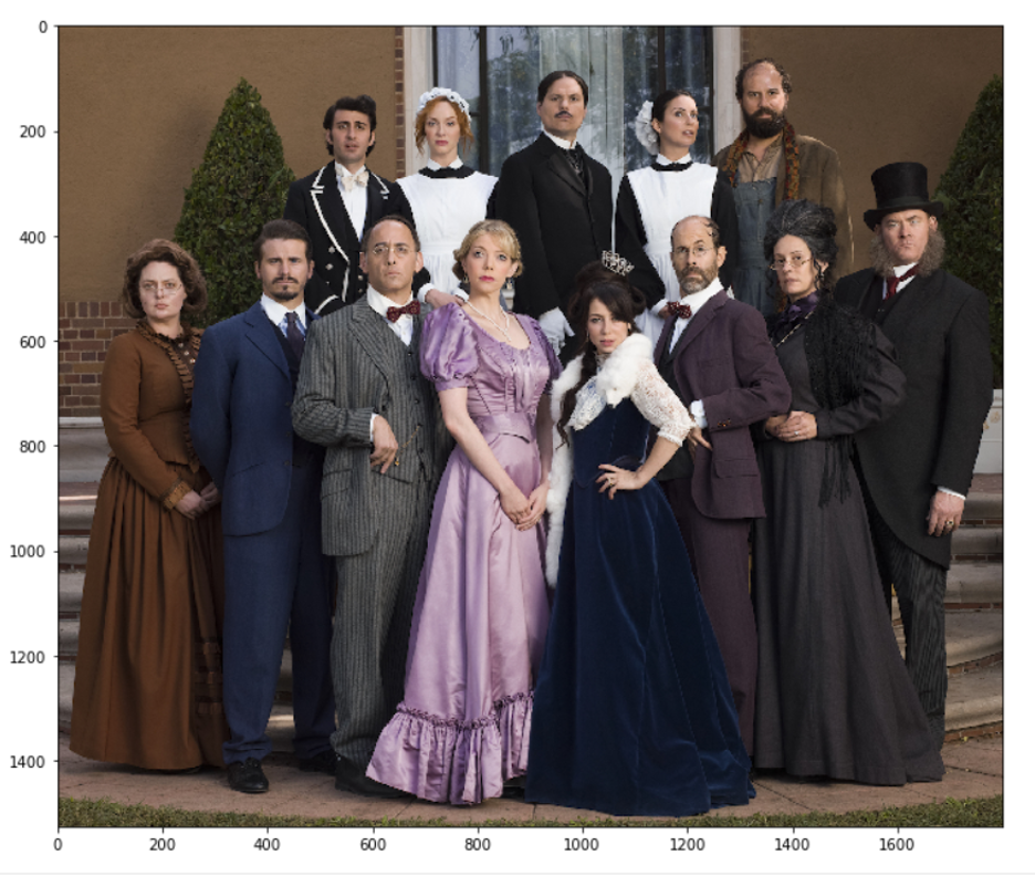
Face Detection
Một chương trình cũ, nhưng vẫn phổ biến để phát hiện khuôn mặt là bộ phân loại tầng Haar; các bộ phân loại này trong thư viện OpenCV và sử dụng các tầng phân loại dựa trên tính năng học cách cô lập và phát hiện các khuôn mặt trong một hình ảnh. bài báo gốc đề xuất cách tiếp cận này ở đây. Và ở đây: OpenCV: Cascade Classifier
# loading in color image for face detection
image = cv2.imread(IMG_PATH+'images/multi_faces.jpg')

# converting to RBG
image = cv2.cvtColor(image, cv2.COLOR_BGR2RGB)

plt.figure(figsize=(20,10))
plt.imshow(image)
# converting to grayscale
gray = cv2.cvtColor(image, cv2.COLOR_BGR2GRAY)

plt.figure(figsize=(20,10))
plt.imshow(gray, cmap='gray')

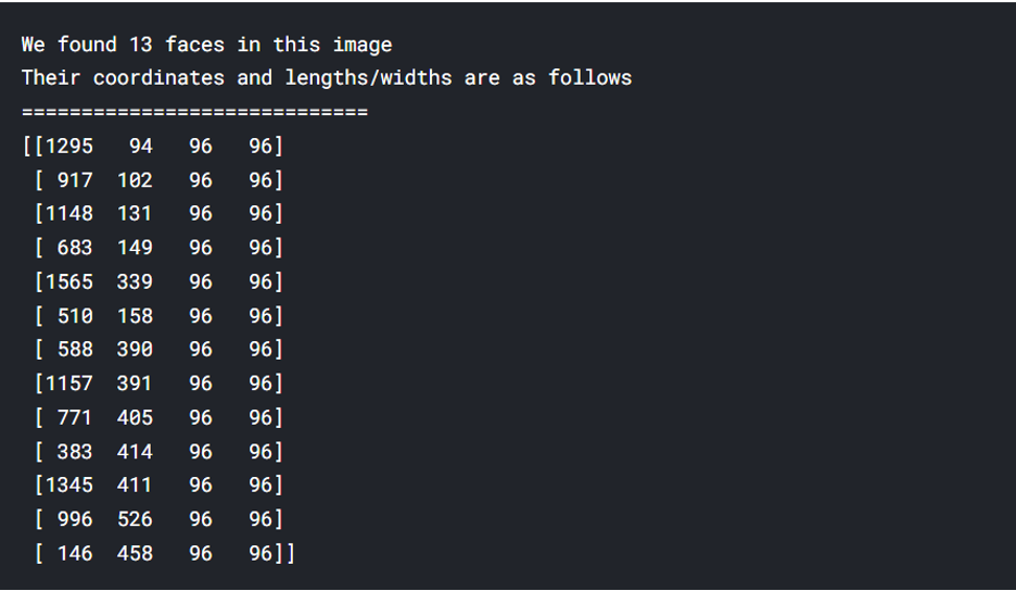
Lưu ý ở các tham số. Có nhiều khuôn mặt được phát hiện được xác định bởi chức năng detectorMultiScale nhằm mục đích phát hiện các khuôn mặt có kích thước khác nhau. Các đầu vào cho chức năng này là: (image, scaleFactor, minNeighbors); bạn thường sẽ phát hiện nhiều khuôn mặt hơn với scaleFactor nhỏ hơn và giá trị minNeighbors thấp hơn, nhưng việc nâng cao các giá trị này thường tạo ra các kết quả khớp tốt hơn. Sửa đổi các giá trị này tùy thuộc vào hình ảnh đầu vào của bạn.
# loading in cascade classifier
face_cascade = cv2.CascadeClassifier('introcv/detector_architectures/haarcascade_frontalface_default.xml')

# running the detector on the grayscale image
faces = face_cascade.detectMultiScale(gray, 4, 6)\

# printing out the detections found
print ('We found ' + str(len(faces)) + ' faces in this image')
print ("Their coordinates and lengths/widths are as follows")
print ('=============================')
print (faces)
# một bản sao của hình ảnh gốc để vẽ biểu đồ phát hiện hình chữ nhật
img_with_detections = np.copy(image)

# lặp lại các phát hiện của và vẽ các box tương ứng của lên trên hình ảnh ban đầu
for (x,y,w,h) in faces:

    cv2.rectangle(img_with_detections,(x,y),(x+w,y+h),(255,0,0),5)

plt.figure(figsize=(20,10))
plt.imshow(img_with_detections)
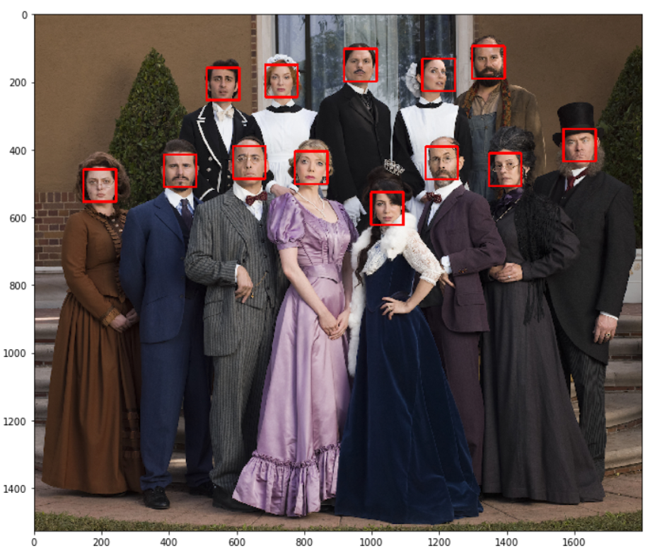
Image Features
Harris Corner Detection
Harris Corner Detection là một thuật toán phát hiện góc thường được sử dụng trong các thuật toán thị giác máy tính để trích xuất các góc và suy ra các đặc điểm của hình ảnh. Nó được giới thiệu lần đầu tiên bởi Chris Harris và Mike Stephens vào năm 1988 sau khi cải tiến máy dò góc của Moravec. So với trước đó, máy dò góc của Harris tính đến sự khác biệt của điểm góc với tham chiếu trực tiếp đến hướng, thay vì sử dụng các bản vá dịch chuyển cho mỗi góc 45 độ và đã được chứng minh là chính xác hơn trong việc phân biệt giữa các cạnh và góc . Kể từ đó, nó đã được cải tiến và áp dụng trong nhiều thuật toán để xử lý trước hình ảnh cho các ứng dụng tiếp theo.
# Read in the image
image = cv2.imread(IMG_PATH+'images/waffle.jpg')

# Make a copy of the image
image_copy = np.copy(image)

# Change color to RGB (from BGR)
image_copy = cv2.cvtColor(image_copy, cv2.COLOR_BGR2RGB)

plt.imshow(image_copy)

gray = cv2.cvtColor(image_copy, cv2.COLOR_RGB2GRAY)
gray = np.float32(gray)

# Detecting corners
dst = cv2.cornerHarris(gray, 2, 3, 0.04)

# Dilating corner image to enhance corner points
dst = cv2.dilate(dst,None)

plt.imshow(dst, cmap='gray')

thresh = 0.1*dst.max()

# Creating an image copy to draw corners on
corner_image = np.copy(image_copy)

# Iterating through all the corners and draw them on the image (if they pass the threshold)
for j in range(0, dst.shape[0]):
    for i in range(0, dst.shape[1]):
        if(dst[j,i] > thresh):
            # image, center pt, radius, color, thickness
            cv2.circle( corner_image, (i, j), 1, (0,255,0), 1)

plt.imshow(corner_image)

Contour Detection
Mỗi contour đều có một số đặc điểm có thể được tính toán, bao gồm diện tích của contour, hướng của nó (hướng mà hầu hết contour hướng vào), chu vi và nhiều thuộc tính khác được nêu trong OpenCV documentation.
image = cv2.imread(IMG_PATH+'images/thumbs_up_down.jpg')

image = cv2.cvtColor(image, cv2.COLOR_BGR2RGB)

plt.imshow(image)

gray = cv2.cvtColor(image,cv2.COLOR_RGB2GRAY)

# Binary thresholded image
retval, binary = cv2.threshold(gray, 225, 255, cv2.THRESH_BINARY_INV)

plt.imshow(binary, cmap='gray')

# Finding contours from thresholded, binary image
contours, hierarchy = cv2.findContours(binary, cv2.RETR_TREE, cv2.CHAIN_APPROX_SIMPLE)

# Drawing all contours on a copy of the original image
contours_image = np.copy(image)
contours_image = cv2.drawContours(contours_image, contours, -1, (0,255,0), 3)

plt.imshow(contours_image)

K-Means Clustering
Phân cụm K-mean là một phương pháp lượng tử hóa vectơ, ban đầu từ xử lý tín hiệu, nhằm mục đích phân chia n quan sát thành k cụm trong đó mỗi quan sát thuộc về cụm có giá trị trung bình gần nhất (cluster centers hoặc cluster centroid), đóng vai trò là nguyên mẫu của cụm. Điều này dẫn đến việc phân vùng không gian dữ liệu thành các ô Voronoi (Voronoi cells). Phân cụm K-mean giảm thiểu các phương sai trong cụm (bình phương khoảng cách Euclide), nhưng không phải khoảng cách Euclid thông thường, đây sẽ là bài toán Weber khó hơn: giá trị trung bình tối ưu hóa sai số bình phương, trong khi chỉ có trung vị hình học giảm thiểu khoảng cách Euclid. Ví dụ, các giải pháp Euclid tốt hơn có thể được tìm thấy bằng cách sử dụng k-medians và k-medoid. Ứng dụng của thuật toán K-mean rất nhiều, trong đó có việc nén dung lượng ảnh mà không làm mất đi quá nhiều chất lượng ảnh (image compression), feature learning, cluster analysis, vector quantization…
image = cv2.imread(IMG_PATH+'images/monarch.jpg')

image = cv2.cvtColor(image, cv2.COLOR_BGR2RGB)

plt.imshow(image)

# Reshaping image into a 2D array of pixels and 3 color values (RGB)
pixel_vals = image.reshape((-1,3))

# Converting to float type
pixel_vals = np.float32(pixel_vals)
# you can change the number of max iterations for faster convergence!
criteria = (cv2.TERM_CRITERIA_EPS + cv2.TERM_CRITERIA_MAX_ITER, 10, 0.2)

k = 3

retval, labels, centers = cv2.kmeans(pixel_vals, k, None, criteria, 10, cv2.KMEANS_RANDOM_CENTERS)

# converting data into 8-bit values
centers = np.uint8(centers)
segmented_data = centers[labels.flatten()]

# reshaping data into the original image dimensions
segmented_image = segmented_data.reshape((image.shape))
labels_reshape = labels.reshape(image.shape[0], image.shape[1])

plt.imshow(segmented_image)

Image Pyramids Image Pyramids (pyramid - Kim tự tháp), là một loại biểu diễn tín hiệu đa tỷ lệ được phát triển bởi cộng đồng xử lý tín hiệu, xử lý hình ảnh và thị giác máy tính, trong đó một tín hiệu hoặc hình ảnh phải được làm mịn và lấy mẫu con lặp lại. Biểu diễn kim tự tháp là tiền thân của biểu diễn không gian quy mô và phân tích đa giải.
image = cv2.imread(IMG_PATH+'images/rainbow_flag.jpg')

image = cv2.cvtColor(image, cv2.COLOR_BGR2RGB)

plt.imshow(image)

level_1 = cv2.pyrDown(image)
level_2 = cv2.pyrDown(level_1)
level_3 = cv2.pyrDown(level_2)

# Displaying the images
f, (ax1,ax2,ax3,ax4) = plt.subplots(1, 4, figsize=(20,10))

ax1.set_title('original')
ax1.imshow(image)

ax2.imshow(level_1)
ax2.set_xlim([0, image.shape[1]])
ax2.set_ylim([0, image.shape[0]])

ax3.imshow(level_2)
ax3.set_xlim([0, image.shape[1]])
ax3.set_ylim([0, image.shape[0]])

ax4.imshow(level_3)
ax4.set_xlim([0, image.shape[1]])
ax4.set_ylim([0, image.shape[0]])

Convolutional Neural Networks
Trong deep learning, mạng nơ-ron phức hợp (CNN, hoặc ConvNet) là một lớp mạng nơ-ron nhân tạo, được áp dụng phổ biến nhất để phân tích hình ảnh trực quan. Chúng còn được gọi là mạng nơ-ron nhân tạo bất biến hoặc bất biến trong không gian (SIANN), dựa trên kiến trúc trọng số chia sẻ của các nhân hoặc bộ lọc tích chập trượt dọc theo các tính năng đầu vào và cung cấp các phản hồi tương đương dịch được gọi là bản đồ đối tượng. Về mặt phản trực giác, hầu hết các mạng nơ-ron tích chập chỉ tương đương, trái ngược với bất biến, đối với phép dịch. Họ có các ứng dụng trong nhận dạng hình ảnh và video, hệ thống khuyến nghị, phân loại hình ảnh, phân đoạn hình ảnh, phân tích hình ảnh y tế, xử lý ngôn ngữ tự nhiên, và chuỗi thời gian tài chính…
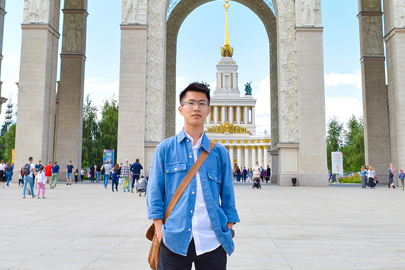
img_path = IMG_PATH+'images/car.png'

bgr_img = cv2.imread(img_path)
gray_img = cv2.cvtColor(bgr_img, cv2.COLOR_BGR2GRAY)

gray_img = gray_img.astype("float32")/255

plt.imshow(gray_img, cmap='gray')
plt.show()

Filters
Một vài filter thường xử dụng để biến đổi hình ảnh qua phép tích chập
filter_vals = np.array([[-1, -1, 1, 1], [-1, -1, 1, 1], [-1, -1, 1, 1], [-1, -1, 1, 1]])
# defining four filters
filter_1 = filter_vals
filter_2 = -filter_1
filter_3 = filter_1.T
filter_4 = -filter_3
filters = np.array([filter_1, filter_2, filter_3, filter_4])
# visualizing filters
fig = plt.figure(figsize=(10, 5))
for i in range(4):
    ax = fig.add_subplot(1, 4, i+1, xticks=[], yticks=[])
    ax.imshow(filters[i], cmap='gray')
    ax.set_title('Filter %s' % str(i+1))
    width, height = filters[i].shape
    for x in range(width):
        for y in range(height):
            ax.annotate(str(filters[i][x][y]), xy=(y,x),
                        horizontalalignment='center',
                        verticalalignment='center',
                        color='white' if filters[i][x][y]<0 else 'black')

Pytorch for Deep Learning
import torch
import torch.nn as nn
import torch.nn.functional as F

# data loading and transforming
from torchvision.datasets import FashionMNIST
from torch.utils.data import DataLoader
from torchvision import transforms
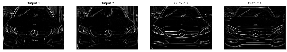
Convolutional layer Single convolutional layer chứa tất cả các bộ lọc đã tạo. Khởi tạo các trọng số trong một lớp phức hợp để có thể hình dung những gì xảy ra sau khi chuyển tiếp qua mạng này!
# neural network with a single convolutional layer with four filters
class Net(nn.Module):

    def __init__(self, weight):
        super(Net, self).__init__()
        # initializing the weights of the convolutional layer to be the weights of the 4 defined filters
        k_height, k_width = weight.shape[2:]
        self.conv = nn.Conv2d(1, 4, kernel_size=(k_height, k_width), bias=False)
        self.conv.weight = torch.nn.Parameter(weight)

    def forward(self, x):
        # calculates the output of a convolutional layer
        # pre- and post-activation
        conv_x = self.conv(x)
        activated_x = F.relu(conv_x)

        # returns both layers
        return conv_x, activated_x

# instantiating the model and setting the weights
weight = torch.from_numpy(filters).unsqueeze(1).type(torch.FloatTensor)
model = Net(weight)

print(model)

>>> Net((conv): Conv2d(1, 4, kernel_size=(4, 4), stride=(1, 1), bias=False))

# helper function for visualizing the output of a given layer
# default number of filters is 4

def viz_layer(layer, n_filters= 4):
    fig = plt.figure(figsize=(20, 20))

    for i in range(n_filters):
        ax = fig.add_subplot(1, n_filters, i+1, xticks=[], yticks=[])
        # grab layer outputs
        ax.imshow(np.squeeze(layer[0,i].data.numpy()), cmap='gray')
        ax.set_title('Output %s' % str(i+1))
# plotting original image
plt.imshow(gray_img, cmap='gray')

# visualizing all filters
fig = plt.figure(figsize=(12, 6))
fig.subplots_adjust(left=0, right=1.5, bottom=0.8, top=1, hspace=0.05, wspace=0.05)
for i in range(4):
    ax = fig.add_subplot(1, 4, i+1, xticks=[], yticks=[])
    ax.imshow(filters[i], cmap='gray')
    ax.set_title('Filter %s' % str(i+1))

# converting the image into an input Tensor
gray_img_tensor = torch.from_numpy(gray_img).unsqueeze(0).unsqueeze(1)

# getting the convolutional layer (pre and post activation)
conv_layer, activated_layer = model(gray_img_tensor)

# visualizing the output of a conv layer
viz_layer(conv_layer)


Pooling Layer
Pooling Layer cung cấp một cách tiếp cận để down sampling feature maps bằng cách tóm tắt sự hiện diện của feature maps trong patchs của feature maps. Hai phương pháp tổng hợp phổ biến là pooling và max pooling tóm tắt sự hiện diện trung bình của một feature và sự hiện diện được kích hoạt nhiều nhất của một feature tương ứng.
# Adding a pooling layer of size (4, 4)
class Net(nn.Module):

    def __init__(self, weight):
        super(Net, self).__init__()
        k_height, k_width = weight.shape[2:]
        self.conv = nn.Conv2d(1, 4, kernel_size=(k_height, k_width), bias=False)
        self.conv.weight = torch.nn.Parameter(weight)
        # defining a pooling layer
        self.pool = nn.MaxPool2d(4, 4)

    def forward(self, x):
        # calculates the output of a convolutional layer
        # pre- and post-activation
        conv_x = self.conv(x)
        activated_x = F.relu(conv_x)

        # applies pooling layer
        pooled_x = self.pool(activated_x)

        # returns all layers
        return conv_x, activated_x, pooled_x

weight = torch.from_numpy(filters).unsqueeze(1).type(torch.FloatTensor)
model = Net(weight)

print(model)

>>>
Net((conv): Conv2d(1, 4, kernel_size=(4, 4), stride=(1, 1), bias=False)
(pool): MaxPool2d(kernel_size=4, stride=4, padding=0, dilation=1, ceil_mode=Fase)


plt.imshow(gray_img, cmap='gray')

# visualizing
fig = plt.figure(figsize=(12, 6))
fig.subplots_adjust(left=0, right=1.5, bottom=0.8, top=1, hspace=0.05, wspace=0.05)
for i in range(4):
    ax = fig.add_subplot(1, 4, i+1, xticks=[], yticks=[])
    ax.imshow(filters[i], cmap='gray')
    ax.set_title('Filter %s' % str(i+1))


# chuyển data thành tensor
gray_img_tensor = torch.from_numpy(gray_img).unsqueeze(0).unsqueeze(1)

conv_layer, activated_layer, pooled_layer = model(gray_img_tensor)

# visualizing the output of the activated conv layer
viz_layer(activated_layer)

# visualizing the output of the pooling layer
viz_layer(pooled_layer)


P/S
Trong khuôn khổ bài viết này, mình đã đề cập tới một số phương pháp thường sử dụng trong việc xử lý ảnh. OpenCV là một thư viện rất mạnh hỗ trợ các hàm xử lý ảnh. Việc xử dụng thành thạo OpenCV sẽ là một lợi thế mạnh trong việc xử lý ảnh và tiền xử lý data raw cho các mô hình Máy học cũng như các mô hình học sâu.
Mình vừa kết thúc phần 1. Phần 2 (từ CNN tới SOTA) mình sẽ cố gắng dành thời gian để viết về nó một cách ngắn và dễ hiểu nhất (mình cũng chưa biết khi nào xong vì nó thực sự quá nhiều và quá dài 🙁). Computer Vision là một lĩnh vực rất rất lớn, trong khuôn khổ 1, 2 bài viết không thể hoàn toàn bao phủ hết về nó, chỉ mong qua bài viết của mình, các bạn có thêm nhiều động lực để tìm hiểu về thị giác máy tính.
Có thể trong quá trình viết có sai sót, hi mọi người cùng sửa chữa để mọi thứ tốt hơn.
Thanks for reading.
Minh!</cite
Useful links/Books:
Computer Vision: Algorithms and Applications (Texts in Computer Science): Szeliski, Richard
(highly recommend vì cuốn sách này tuy cực kỳ hàn lâm nhưng nó là cuốn sách rất rất hay)
Rapid Object Detection using a Boosted Cascade of Simple Features
OpenCV Python Tutorial - GeeksforGeeks
15 OpenCV Projects Ideas for Beginners to Practice in 2021 (projectpro.io)
Start Here with Computer Vision, Deep Learning, and OpenCV - PyImageSearch
CS231n Convolutional Neural Networks for Visual Recognition